Introduction
phlite is a Rust library for computing persistent homology of filtered chain complexes, with Python bindings
for three kinds of input. It began as a way to compute grounded persistent path homology of digraphs
(GrPPH), and grew into a general framework in which the same reduction algorithms run on any
filtered chain complex you can describe, whether or not it fits in memory.
The idea: matrices you never store
Every persistent homology computation boils down to reducing a big sparse matrix: the boundary matrix of the filtration, or its transpose. Most libraries (PHAT, LoPHAT, Dionysus, GUDHI’s matrix reductions, …) want that matrix stored, column by column, in filtration order, with integer row and column indices.
That is often impossible. The Vietoris–Rips complex of 1000 points up to dimension 2 has 166 million triangles and 41 billion tetrahedra; the path complex of a dense digraph is worse. Ripser’s great insight was that you never need to store the matrix: a column can be recomputed whenever it is needed, from a compact description of the cell (a few integers), and most columns are never needed at all.
phlite turns that insight into a library. You describe your matrix as an oracle: a function that, given a
column’s label (any type you like, not necessarily an integer), produces that column’s entries on demand.
flowchart LR
    U["Your filtration<br/>(points, a digraph, an image...)"] --> O["Matrix oracle<br/>column(c) -> entries"]
    O --> A["Reduction algorithm<br/>(standard, clearing, parallel)"]
    A --> B["Barcode<br/>+ representatives"]
Everything else is optional help you can give the algorithms, and each piece unlocks a further optimisation:
| You provide | phlite can then |
|---|---|
| the column oracle, a filtration on rows, an ordered column basis | compute persistence with the standard algorithm |
| the basis split by dimension | use clearing |
| the transpose (or just “first column in each row”) | recognise apparent pairs, skip most columns entirely |
| a fast way to find a column’s pivot | finish most columns without building them (emergent pairs) |
| columns already sorted | add them without sorting |
| dense integer labels, and row ranks | use vectors instead of hash maps, and PHAT-style pivot columns |
The tutorial walks through these one at a time on a concrete example.
What is in the box
phlite: the core library: the matrix traits and adaptors, the reduction algorithms (standard, clearing, and a lock-free parallel clearing after Morozov and Nigmetov), four representations of the column being reduced, a column cache, and helpers that turn a reduction into a barcode with representatives, by homology or cohomology.phlite_rips: Vietoris–Rips persistence, with Ripser’s and giotto-ph’s optimisations, as a Rust crate, a CLI and thephlite_ripsPython package.phlite_grpph: grounded persistent path homology of weighted digraphs, as a crate and thephlite_grpphPython package.phlite_py: thephlitePython package, for explicit filtered chain complexes you build yourself: from integer columns, CSC arrays, or your own Python objects as cells. It is a drop-in alternative to PHAT and LoPHAT that also gives representatives and works over Z/p.
How fast?
Measured on one thread against the specialised tools (see the benchmarks):
- Vietoris–Rips: on a par with ripser and giotto-ph, faster in dimension 2 on random points.
- GrPPH: 25–100× faster than grpphati.
- Explicit complexes: 7–13× faster than PHAT on Rips complexes, faster on sparse cell complexes, level on dense boundaries and meshes, and within about 10–20% on large cubical complexes.
How to read this book
- Background recaps persistent homology as matrix reduction, using one small example that the rest of the book keeps coming back to.
- How phlite is built explains the oracle traits.
- The chapters on reduction algorithms and column representations explain every algorithm and trick: how it works, why it helps, and when it doesn’t.
- Inside phlite covers the lower-level engineering, and where the time actually goes.
- The tutorial builds a filtration of your own in Rust, step by step.
- The Python chapters document the three packages, with example notebooks. (The API reference is generated from their docstrings.)
- The playground runs phlite in your browser (compiled to WebAssembly, on all your cores): point clouds, images, weighted networks and chain complexes, with their barcodes and representatives drawn on the data.
Persistent homology in one chapter
This chapter recaps just enough persistent homology to follow the algorithms, through one running example. For a proper introduction see Edelsbrunner and Harer’s Computational Topology, or Otter et al.’s A roadmap for the computation of persistent homology (see references).
Filtrations
A filtered chain complex is a chain complex whose cells appear one at a time. Each cell has a filtration value (the time it appears), and every face of a cell must appear no later than the cell itself. Here is the running example: four vertices, five edges and a triangle.

The running example. At t = 4 the triangle abc fills in the loop a–b–c.
Listing the cells by filtration value (breaking ties by a fixed order), we get a filtration order:
| index | 0 | 1 | 2 | 3 | 4 | 5 | 6 | 7 | 8 | 9 |
|---|---|---|---|---|---|---|---|---|---|---|
| cell | a | b | c | ab | bc | ac | d | cd | bd | abc |
| value | 0 | 0 | 1 | 1 | 1 | 2 | 2 | 3 | 3 | 4 |
Persistence
As cells appear, homology classes (connected components in dimension 0, loops in dimension 1, voids in dimension 2, …) are born and later die. Each class gives a bar from its birth to its death: the barcode.
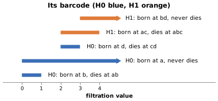
The barcode: two components and a loop die; one component and one loop never do.
Reading it off the filtration:
aandbare born at 0; the edgeabmerges them at 1, so one of the two components dies (by convention the younger one,b).cis born at 1 and dies at 1, whenbcjoins it to the rest: a bar of length zero, which is not drawn.accloses the loop a–b–c at 2; the triangleabcfills it at 4.dis born at 2 and dies at 3.bdcloses another loop at 3 (b–c–d), which nothing ever fills: an essential (infinite) bar.
Persistence by matrix reduction
The boundary matrix \(D\) has a column and a row for every cell, in filtration order; column \(j\) holds the faces of cell \(j\). Over \(\mathbb{Z}/2\) the entries are just 0 and 1.
The pivot (or low) of a column is its last non-zero entry: the face that appeared most recently. We reduce \(D\) by adding columns left to right until no two columns share a pivot, recording the additions in \(V\), so that
\[ R = D V \]
with \(V\) upper triangular. Then the pairing can be read straight off \(R\):
- if column \(j\) of \(R\) has pivot \(i\), the class born at cell \(i\) dies at cell \(j\): a pair \((i, j)\);
- if column \(j\) of \(R\) is zero, cell \(j\) gives birth to a class; if no column has pivot \(j\), that class never dies (it is essential).
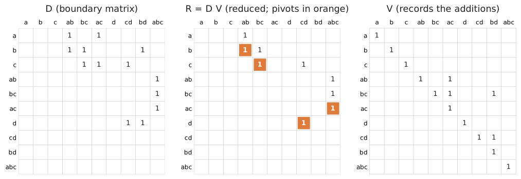
D, its reduction R = DV (pivots in orange) and V. The pairs are (b, ab), (c, bc), (d, cd) and (ac, abc).
Different reductions give different \(R\) and \(V\), but always the same pairs (the pairing uniqueness lemma).
That is what lets phlite choose freely between algorithms, column representations and orders of work: they all
give the same barcode.
Columns of \(R\) and \(V\) are also representatives: for a pair \((i, j)\), column \(j\) of \(R\) is a cycle born at \(i\) that becomes a boundary at \(j\); for an essential class born at \(i\), column \(i\) of \(V\) is a cycle born at \(i\).
Reducing a column
Reducing one column means repeatedly finding its pivot and, if an earlier column owns the same pivot, adding that
column. Here is column ac:
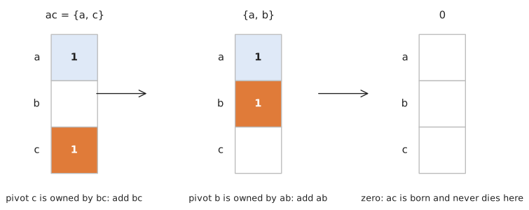
Reducing ac: two additions, after which it is zero, so ac gives birth to a loop.
Every algorithm in phlite is built from these two operations: pop the pivot and add a column. How they are done
is the subject of the column representations; which columns get reduced, and in what
order, is the subject of the reduction algorithms.
Representing a filtration in phlite
phlite doesn’t need you to number your cells or store \(D\). Cells can be labelled by any type (a simplex packed
into an integer, a path in a digraph, a pair of pixel coordinates), and the filtration order is the order on
(filtration value, label). Columns are produced on demand by your oracle.
Homology or cohomology?
There are two matrices you can reduce to get the same barcode.
- Homology reduces the boundary matrix \(D\): columns are cells, entries are their faces.
- Cohomology reduces the coboundary matrix: columns are cells, entries their cofaces. Put in the right order (both cells and cofaces in reverse filtration order) this is the anti-transpose \(D^\perp\) of \(D\).
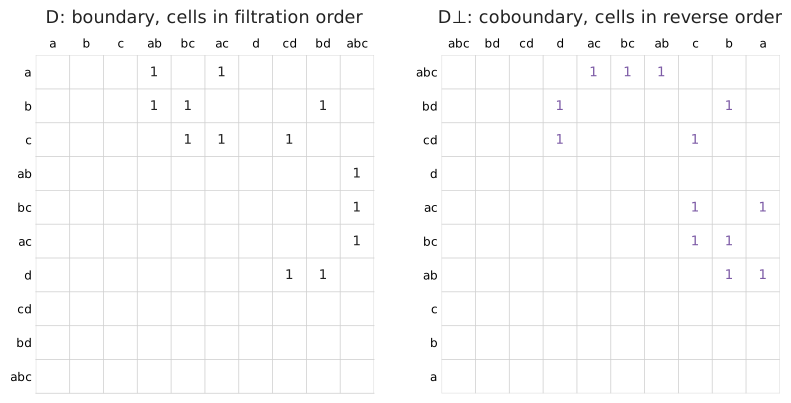
The anti-transpose flips D about its anti-diagonal: rows and columns swap, and both are reversed.
The pairs of \(D^\perp\) are exactly the pairs of \(D\), with birth and death swapped (de Silva, Morozov and
Vejdemo-Johansson). So phlite reduces whichever is cheaper and reports bars in homology conventions either way.
Why cohomology is usually faster
Ripser popularised cohomology because, combined with clearing, it does far less work on filtrations that grow quickly with dimension, like Vietoris–Rips:
- Clearing works in the cheap direction. With cohomology the dimensions are reduced from low to high, and the pairs found in dimension \(d\) clear columns of dimension \(d + 1\), the larger dimension, which has by far the most columns. With homology the pairs clear columns of the smaller dimension.
- No need to enumerate the top dimension. To compute \(H_d\) by cohomology you need columns only up to dimension \(d\); the cells of dimension \(d + 1\) appear only as rows, produced lazily as cofaces. Homology needs every \((d+1)\)-cell as a column. For Rips in dimension 2 that is the difference between enumerating the triangles and enumerating the tetrahedra.
- Apparent pairs are found from the cheap end. Most columns of a Rips coboundary are finished by emergent pairs without being built.
When homology is better
- When you want representatives cheaply. Homology gives cycle representatives directly (columns of \(R\) and
\(V\)). Cohomology gives cocycles;
phlitegets cycles from a cohomology computation with a second, much smaller reduction, the involution, which costs extra. - When columns of the boundary are short and the complex is not much bigger in the next dimension. For explicit cell complexes and some cubical complexes the two are close; in the benchmarks homology was about 7% faster on a cubical complex of random noise, but slower on the others, and about 3× slower on random cell complexes.
- For relative cohomology you can reduce \(D\) in the other direction:
phlite’sreverseadaptor gives the anti-transpose of any matrix.
Every barcode function and Python package takes a method ("cohomology" by default, or "homology").
Matrix oracles
phlite’s central abstraction is the matrix oracle: a matrix you can ask for one column at a time, which need not
be stored anywhere. The traits are in phlite::matrices, and layer up like this:
flowchart TD
    MO["MatrixOracle<br/><i>column(c): the entries of column c</i>"]
    RF["HasRowFiltration<br/><i>filtration_value(r) + optional hooks</i>"]
    CB["HasColBasis<br/><i>the columns to reduce, in order</i>"]
    SB["HasSplitColBasis<br/><i>...split by dimension</i>"]
    TR["HasTranspose<br/><i>the transpose (optional)</i>"]
    RED["Reduction algorithms"]
    MO --> RF
    MO --> CB --> SB
    MO --> TR
    RF --> RED
    SB --> RED
    TR -. "apparent pairs,<br/>involution" .-> RED
MatrixOracle: the columns
pub trait MatrixOracle {
    type CoefficientField: NonZeroCoefficient; // e.g. Z2, or ZP<3>
    type ColT: BasisElement;                  // labels of columns
    type RowT: BasisElement;                  // labels of rows

    fn column(&self, col: Self::ColT) -> impl Iterator<Item = (Self::CoefficientField, Self::RowT)>;
}
That is the only required method. Labels can be any type that is Ord + Clone (and marked as a
BasisElement): Ripser-style packed simplex indices, paths in a digraph, coordinates. The
order on labels breaks ties between cells with the same filtration value.
Why an iterator? So that columns are produced lazily, in whatever order is convenient, and never stored. The
algorithms consume them with internal iteration (for_each), so chained and flattened iterators cost nothing.
Coefficients are a type, not a runtime value: Z2 is zero-sized, so a column over Z/2 is just its row labels and
the arithmetic compiles away. ZP<P> covers small primes.
HasRowFiltration: the order
pub trait HasRowFiltration: MatrixOracle {
    type FiltrationT: FiltrationValue; // Ord + Clone, e.g. NotNan<f64>
    fn filtration_value(&self, row: Self::RowT) -> Self::FiltrationT;
    // ... and optional hooks, below
}
Entries are ordered by (filtration value, row label), and the pivot of a column is its largest entry. If you
have no filtration (plain homology) use with_trivial_filtration(); if the filtration is a function, attach it with
with_filtration(f).
The optional hooks
Each has a correct default; overriding it unlocks an optimisation.
| Hook | Default | Override it to… |
|---|---|---|
column_with_filtration | column + filtration_value per entry | compute a column’s filtration values together |
column_pivot / column_min | scan the whole column | find the pivot without visiting every entry (emergent pairs) |
sorted_column | None | hand over columns already sorted, so they aren’t sorted again (merged columns) |
first_column_in_row / last_column_in_row | None | recognise apparent pairs |
row_ranks | None | give each row’s position in filtration order, for pivot columns |
same_filtration_value | compare filtration_values | compare the real values when FiltrationT is finer than the filtration (explicit complexes) |
HasColBasis and HasSplitColBasis: which columns
The matrix says what each column is; the basis says which columns to reduce, and in which order (filtration
order). Clearing needs it split by dimension. The usual way is to build a SplitBasis (one vector of labels, plus
the offset where each dimension starts) and attach it:
let basis = SplitBasis::from_dimensions([vertices, edges, triangles]); // each sorted by filtration
let d = my_boundary.with_basis(basis);
You only need a basis for the columns. Rows are produced by the oracle and never enumerated, which is why cohomology never builds the top-dimensional cells (see Homology or cohomology?).
A basis may also leave cells out: the clearing algorithms don’t need the cells of zero-length apparent pairs, which for Vietoris–Rips is nearly all of them.
HasTranspose
Attach the transpose with with_transpose(t) (for a coboundary, the boundary, and vice versa). It provides
first_column_in_row and last_column_in_row (the pivot and minimum of the transpose’s column), which is what
apparent pairs need, and it is what the involution
reduces to compute representatives from cohomology.
BasisElement: labels
pub trait BasisElement: Ord + Clone {
    const DENSE_INDEX: bool = false;
    fn dense_index(&self) -> usize { unimplemented!() }
    fn from_dense_index(index: usize) -> Self { unimplemented!() }
}
If your labels are (or map injectively to) small integers, set DENSE_INDEX and the reduction’s
bookkeeping uses plain vectors instead of hash maps. The choice is a constant, so the
other branch compiles away.
Adaptors
Methods on MatrixOracle wrap a matrix to add or change something, without copying it:
| Adaptor | Gives |
|---|---|
with_filtration(f), with_trivial_filtration() | a HasRowFiltration |
with_basis(b) | a HasColBasis (and HasSplitColBasis for a SplitBasis) |
with_transpose(t) | a HasTranspose, and apparent pairs |
reverse() | the anti-transpose: the order on rows and columns reversed (labels wrapped in Reverse) |
consolidate() | columns with repeated rows summed |
using_col_basis_index() | columns labelled by their position in the basis |
combinators::product(a, b) | the product of two oracles (e.g. R = D V) |
Adaptors forward the optional hooks where that makes sense; reverse swaps the “first/last” and “pivot/min” ones,
so a coboundary that knows its smallest entry is fast after reversing too.
Wrappers also work on references (&M is a matrix if M is), so you can keep the original and reduce a view of it.
From a matrix to a barcode
There are two levels of API.
Low level: reduction
Each algorithm is a value implementing ReductionAlgorithm. Configure it, then call reduce (giving \(V\) and
the diagram) or diagram (just the pairs, which can be much cheaper):
use phlite::reduction::{Clearing, ReductionAlgorithm};
use phlite::columns::HeapColumns;

let reduction = Clearing::new()
    .with_columns(HeapColumns)   // how to represent the column being reduced
    .cache_columns(false)        // don't keep columns of D
    .reduce(&matrix);
// reduction.v: an oracle for V; reduction.diagram: (birth, death) pairs and essential columns| Algorithm | Notes |
|---|---|
Standard | reduces every column, in order |
Clearing | dimension by dimension, clearing; apparent and emergent pairs; optionally storing R |
ParallelClearing | clearing with each dimension reduced on many threads (Clearing::new().parallel()) |
The diagram is in terms of columns of the matrix you reduced. If you reduced a reversed coboundary, the labels are
wrapped in Reverse, and births and deaths are swapped relative to homology.
High level: barcode
phlite::barcode turns a matrix into Bars in homology conventions, with filtration values, and optionally a
representative cycle for each:
use phlite::barcode::{self, Algorithm};

// Homology: reduce the boundary matrix (with its basis and, ideally, its transpose)
let bars = barcode::homology(boundary, Algorithm::default(), /* representatives */ true);

// Cohomology: reduce the (anti-transposed) coboundary, usually much faster
let bars = barcode::cohomology(coboundary, Algorithm::default());

// Cohomology with cycle representatives, via the involution (needs the transpose attached)
let bars = barcode::cohomology_with_involution(coboundary, Algorithm::default());
flowchart LR
C["coboundary<br/>+ basis + transpose"] -->|reverse| AT["anti-transpose"]
AT -->|reduce| DG["diagram<br/>(cohomology pairs)"]
DG -->|swap birth/death,<br/>add values| BARS["bars"]
DG -.->|"deaths + essential births"| INV["involution:<br/>small homology reduction"]
INV -.->|"columns of R and V"| BARS
Algorithm wraps the three algorithms (Algorithm::Standard(..), Algorithm::Clearing(..),
Algorithm::ParallelClearing(..)), so a caller can pick one at run time.
Bars of length zero are omitted: in most filtrations there are far more of them than of anything else, and they carry no information. The clearing algorithms avoid even recording most of them (see skipping zero-length apparent pairs).
The standard algorithm
for j in columns, in filtration order:
    while column j is non-zero and some earlier column k has the same pivot:
        add (a multiple of) column k to column j       # and record it in V
    if column j is non-zero: column j owns its pivot
This is the textbook algorithm (Edelsbrunner, Letscher and Zomorodian), and phlite::reduction::Standard implements
it with no optimisations: it builds every column in full and needs the full column basis.
let reduction = Standard::new().reduce(&matrix);How it works in phlite
- A pivot table maps each owned pivot (a row label) to its column (
low_inverse). - The column being reduced is a working column with two operations, pop the pivot and add a column; how it is stored is a column representation.
- Only \(V\) is stored, as sparse columns. To add column \(k\) of \(R = DV\), the algorithm adds the column of \(D\) for every term of \(V_k\) (see storing R for the alternative).
When to use it
- As a reference. It is the simplest and the easiest to trust, and the tests compare everything else against it.
- Small matrices, where the bookkeeping of the cleverer algorithms costs more than it saves.
- When the basis can’t be split by dimension, since clearing needs that.
It is slow on anything large: it reduces every column, including the many that clearing would skip, and it can’t
use apparent pairs, so it needs every cell in the basis (phlite_rips gives it the full basis for that reason).
Clearing
Clearing (Chen and Kerber’s “twist”) uses a fact about the pairs: if \((i, j)\) is a pair, then cell \(i\) gives birth to a class, so column \(i\) of \(R\) will be zero. There is no need to reduce it.
So reduce the dimensions in the right order and every pair found in one dimension clears a column of the next:
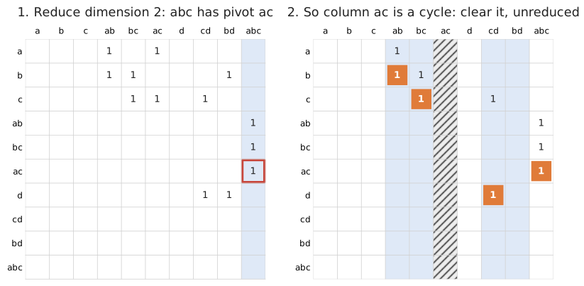
Homology of the running example. Reducing dimension 2 pairs ac with abc, so column ac (hatched) is set to zero without being reduced. Its reduction would have taken two additions.
phlite::reduction::Clearing does this dimension by dimension:
flowchart TD
    S["for each dimension d (in the matrix's direction)"] --> C{"column j paired<br/>in the previous dimension?"}
    C -- yes --> Z["cleared: R_j = 0,<br/>V_j = the other column of R"]
    C -- no --> P{"pivot unclaimed?"}
    P -- yes --> F["finished without building<br/>(emergent / apparent pair)"]
    P -- no --> RED["reduce the column"]
    RED --> REC["record the pair or the birth"]
    F --> REC
    Z --> N["next column"]
    REC --> N
The direction is detected from the matrix: for a boundary matrix the pivots of dimension \(d\) lie in dimension
\(d - 1\), so dimensions are reduced from the top down; for a (reversed) coboundary from the bottom up. You can fix it
with with_dimension_order.
For representatives the cleared column still needs a \(V\) column; it is \(R_j\) of the column it was paired with,
which phlite keeps a reference to rather than copying (ClearedReductionMatrix).
When it helps
- Almost always. It saves the reduction of every column that gives birth to a class which later dies, which is often the most expensive kind.
- Most with cohomology: the cleared columns are then the cells of the higher dimension, by far the most numerous (see Homology or cohomology?).
When it doesn’t
- It needs the column basis split by dimension (
HasSplitColBasis). - With homology the cleared columns are in the smaller dimension, so it saves less.
- The pairs of each dimension are kept until the next dimension is done, a little memory.
Clearing is also the framework the other tricks plug into: apparent and emergent pairs, storing R and the parallel version all build on it.
Apparent and emergent pairs
Most columns of most filtrations need no reduction at all. These two tricks, both from Ripser (Bauer), finish such columns without reducing them, and often without even building them.
Apparent pairs
A pair \((r, c)\) is apparent if
- \(r\) is the pivot of column \(c\) (the youngest face of \(c\)), and
- \(c\) is the first column with an entry in row \(r\) (the oldest coface of \(r\)).
Then \((r, c)\) is a persistence pair, whatever else is in the matrix: no earlier column can have pivot \(r\) (they have no entry in row \(r\)), so column \(c\) needs no reduction and owns \(r\).
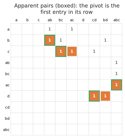
In the running example every pair is apparent (boxed): each pivot is the first entry in its row. Only ac and bd, which give birth to loops, need reducing.
Recognising one takes two lookups: the pivot of \(c\), then the first column in row \(r\), which is the
minimum of row \(r\)’s column in the transpose. So phlite recognises apparent pairs when the matrix provides
first_column_in_row, which with_transpose does.
They need no storage. An apparent pair never changes, so it needn’t go in the pivot table: when another column later hits pivot \(r\), its owner \(c\) can be recomputed (first column in row \(r\), then check its pivot is \(r\)). For Vietoris–Rips, where nearly every pair is apparent, that keeps the pivot table tiny.
Zero-length apparent pairs
If \(r\) and \(c\) also have the same filtration value, the pair is a bar of length zero, which the barcode drops
anyway. The clearing algorithms then don’t even record it (skip_zero_apparent_pairs, on by default). In many
filtrations (lower-star filtrations of images, Vietoris–Rips) these are the vast majority of pairs, so recording
them would dominate the time and memory.
Leaving them out of the basis
Better still, a cell in a zero-length apparent pair can be left out of the column basis entirely, as long as the
matrix can still find it as an owner. phlite_rips does this (build_reduction_bases), and since nearly every Rips pair is a
zero-length apparent pair, it keeps only a small fraction of the edges and triangles. The standard algorithm can’t recompute owners,
so it needs the full basis.
Emergent pairs
A column whose pivot nobody owns yet needs no reduction either: it just claims its pivot. If the matrix can find a
column’s pivot without enumerating the column (the column_pivot hook), the algorithm never builds that column.
For Rips cohomology this is very effective: cofacets can be enumerated in order, and the first cofacet with the simplex’s own diameter is its pivot (no cofacet can have a smaller diameter), so the search usually stops after a step or two. Bauer calls these pairs emergent.
When they help, and when they don’t
| Helps when | Doesn’t when | |
|---|---|---|
| Apparent pairs | the transpose is cheap (oracle or stored), and most pairs are apparent: Rips, lower-star filtrations, cubical complexes | the transpose is expensive to query and few pairs are apparent |
| Skipping zero-length ones | most pairs have length zero | (no downside; turn it off only to see every pair) |
| Leaving them out of the basis | you build the basis yourself and can test apparentness cheaply | you need the standard algorithm, or the full basis anyway |
| Emergent pairs | column_pivot can stop early (enumerating in order with a bound) | the pivot can only be found by scanning (then the default does exactly that) |
For explicit complexes (the phlite Python package) the transpose is stored, so apparent pairs cost two array
lookups, and phlite_py goes one step further: since every cell is in the basis, the pivot table stores apparent pairs
too, so that finding an owner is one lookup (see bookkeeping).
Storing R, or recomputing it from V
When column \(j\) of \(R\) is needed to cancel a pivot, there are two ways to get it.
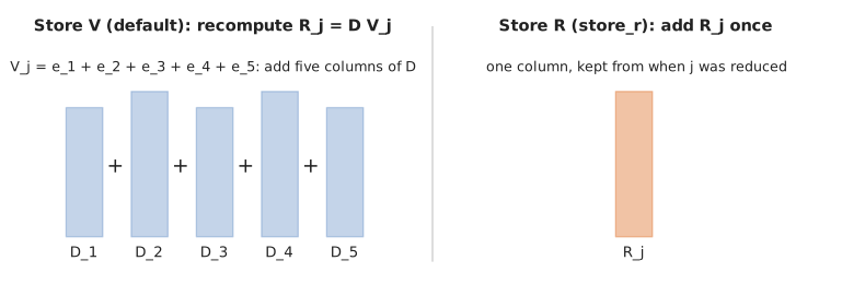
Store V, recompute R (the default)
\(V_j\) is stored (sparse), and \(R_j = D V_j\) is rebuilt by adding the column of \(D\) for every term of \(V_j\). This is what Ripser does.
- Good when \(V\) stays short: for Vietoris–Rips cohomology almost every pair is apparent, \(V_j = e_j\), and “recomputing” \(R_j\) is just generating one column of \(D\), which the oracle does cheaply.
- Memory-light: \(V\) is usually much sparser than \(R\), and the columns of \(D\) are never stored.
- Bad when \(V\) gets long: on dense matrices or cubical complexes a column of \(V\) can have hundreds of terms, and every use of \(R_j\) re-adds hundreds of columns of \(D\).
Store R (store_r)
Clearing::new().store_r(true) keeps each reduced column \(R_j\) (from its pivot down) when it is first reduced, for
the rest of its dimension, and adds it as one column. This is what PHAT does.
- Good when columns need many additions: dense boundary matrices, cubical complexes, homology of cell complexes. On those it is several times faster.
- Bad for memory when \(R\) is much denser than \(V\).
- No gain for Vietoris–Rips cohomology, where almost nothing is reduced.
Apparent pairs and columns that needed no reduction are still never stored: their \(R_j = D_j\) comes straight from the oracle.
Not tracking V at all
When only the diagram is wanted (no representatives), and \(R\) is stored, nothing needs \(V\), so Clearing’s
diagram() doesn’t track it. On dense matrices building \(V\) was most of the remaining work.
Who uses what
| default | |
|---|---|
phlite (Rust) | store V |
phlite_rips, phlite_grpph | store V |
phlite (Python, explicit complexes) | store R (serial clearing) |
Parallel clearing
Clearing::new().parallel() reduces each dimension on many threads, after Morozov and Nigmetov’s lock-free
reduction (Towards lockfree persistent homology), organised much as in giotto-ph. It needs the parallel feature
(on in the Python packages).
How it works
Dimensions are still done one after another (clearing needs the previous dimension’s pairs), but within a dimension:
flowchart LR
    subgraph P1["1. Classify (parallel, no shared state)"]
        A1["cleared"]
        A2["zero"]
        A3["apparent pair"]
        A4["needs reduction"]
    end
    subgraph P2["2. Reduce (parallel, lock-free)"]
        B1["threads take columns;<br/>steal pivots owned by<br/>columns to their right"]
    end
    subgraph P3["3. Read off pairs"]
        C1["per-thread lists<br/>+ reduced columns"]
    end
    P1 --> P2 --> P3
- Classify every column in parallel: cleared, zero, apparent, or needing reduction. Results go into per-thread vectors, so this phase shares nothing. Typically only a small fraction of columns need reduction, and only they get any shared state.
- Reduce those columns concurrently. A thread reduces a private copy of its column; when it meets a pivot owned by a column to its right (later in filtration order), it publishes its own column, steals the pivot, and carries on reducing the displaced column instead. Every column ends up owning a pivot or reduced to zero, and by the pairing uniqueness lemma the pairs are the same as the serial algorithm’s.
- Read off the pairs.
The pivot table is a concurrent map keyed by row label, never by row index, so the row space is never enumerated (the main saving of cohomology survives). Published columns are snapshots of \(V_j\) with their pivot cached.
There are two storage backends:
storage | Pivot table | Published columns | |
|---|---|---|---|
locking (default) | DashMap (sharded read–write locks) | Arc behind a lock | robust, slightly faster on few threads |
lock-free (feature lock-free) | papaya map, compare-and-swap | ArcSwap slots | no thread ever waits on another |
When it helps
- Large dimensions with many columns needing reduction: GrPPH, Vietoris–Rips in dimension 2, large explicit complexes. The classify phase alone parallelises the expensive “is this column apparent?” checks.
When it doesn’t
- Small inputs: thread start-up and the concurrent maps cost more than they save.
- When almost nothing needs reduction: the work is then in classification, which serial clearing also does quickly.
- It doesn’t support storing R or pivot columns (each column is reduced in a fresh working column), so for explicit cubical or dense complexes serial clearing with both is usually faster than parallel.
- Memory: each thread has its own working column, and published columns are kept as snapshots.
Use it with Algorithm.parallel(threads) in Python, or Clearing::new().parallel().in_pool(&pool) in Rust to run on
your own rayon pool.
Representatives and the involution
A representative of a bar is a cycle that is born at the bar’s birth and (for a finite bar) becomes a boundary exactly at its death.
From homology: for free
Reducing the boundary matrix gives them directly:
- for a pair \((b, d)\), column \(d\) of \(R = DV\): a cycle with pivot \(b\) that is the boundary of \(V_d\), a chain present at \(d\);
- for an essential class born at \(b\), column \(b\) of \(V\): a cycle (\(R_b = 0\)) with leading term \(b\).
From cohomology: the involution
Cohomology is usually much faster, but its reduction gives cocycles. To get cycles,
barcode::cohomology_with_involution uses Čufar’s involuted persistence:
- Compute the pairs by cohomology, as fast as usual.
- Run a homology reduction on the boundary matrix (the coboundary’s transpose), but only of the columns that matter: the death cells of finite bars and the birth cells of essential bars.
- Read representatives off that small reduction’s \(R\) and \(V\), as above.
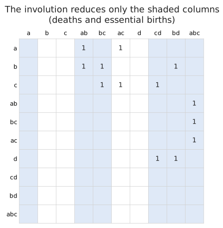
For the running example only six of ten columns are reduced: the deaths ab, bc, cd and abc, and the essential births a and bd.
Why is that enough? Reducing a column only ever adds earlier columns that own a pivot, and every column that owns a pivot is a death, so the death columns are closed under the reduction. Zero-length pairs are deaths too, and may be missing from the diagram (they are skipped), so this reduction keeps apparent pairs switched on: their owners are recognised through the coboundary, without being in the basis.
Costs and trade-offs
- Good when bars are few compared with cells, as is typical: the second reduction touches only the death columns, and nearly all of those are apparent pairs that need no work.
- Costs a homology reduction, which can be the slow direction, and needs the transpose (the boundary) to be available. On filtrations with very many bars (random point clouds in high dimension) it can cost as much as the cohomology itself.
- The reduction in step 2 uses a restricted basis, so it must not assume that every column is in the basis: in
particular phlite_py’s single-lookup pivot table (
full_basis) is switched off for it (see bookkeeping). A bug where it wasn’t was found by the fuzz tests.
Representatives in phlite are reported as lists of (cell, coefficient) in decreasing filtration order, so the
birth cell comes first.
The working column
Whatever the algorithm, reducing a column means repeating two operations on a working column \(R_i = D V_i\):
- pop the pivot: find its largest entry (summing entries with the same row, and moving on when they cancel);
- add a column: add a multiple of a column of \(D\) (or a stored column of \(R\)) to it.
flowchart LR
    W["working column R_i"] -->|pop pivot r| O{"r owned by<br/>column j?"}
    O -- no --> DONE["R_i owns r: done"]
    O -- yes --> ADD["add (a multiple of) R_j<br/>= add columns of D"]
    ADD --> W
How the working column is stored is its representation, a type implementing ColumnRepresentation, chosen
with with_columns on any algorithm:
Clearing::new().with_columns(PivotColumns)Every representation gives the same pairs; only the time and memory differ. The difference can be large: on some inputs the best is 30× faster than the worst. There are four:
| Representation | Idea | Analogue |
|---|---|---|
HeapColumns | every term on one heap | Ripser |
MergedColumns (default) | lazily merge sorted columns, one heap slot per column | |
SortedColumns | one sorted vector, batches merged in | PHAT’s vector_vector |
PivotColumns | a dense array over all rows, plus a bit tree | PHAT’s bit_tree_pivot_column |
Separately, a column cache can keep the columns of \(D\) that get added, sorted, so they are neither recomputed nor re-sorted. Choosing summarises when each wins.
Heap columns
HeapColumns pushes every term of every column added onto one heap (BHCol), and pops from the top, summing
terms with the same row as they surface. This is the classic approach, and what Ripser does.
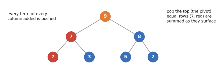
The heap holds every term added, including both copies of row 7, which cancel when they reach the top.
phlite uses a 4-ary heap: half the depth of a binary heap, with each node’s children next to each other in
memory, which matters once the heap outgrows the cache (an 8-ary heap was slower).
Good
- No sorting at all. Columns of \(D\) go in as the oracle produces them.
- Little memory when few, short columns are added: just the terms.
- On Vietoris–Rips cohomology, where columns are short and few are added per column, it matches merged columns
with less memory, which is why it is
phlite_rips’ default.
Bad
- Many terms added: the heap holds every term, cancelled or not, including all those far below the eventual pivot. Each push and pop costs \(O(\log n)\) in the heap’s size, and once it outgrows the cache every operation slows down.
- So it is slow for GrPPH, cubical complexes and dense matrices (3–4× slower than merged columns on GrPPH).
Merged columns
MergedColumns (the default in the Rust library and phlite_grpph) never builds the working column. It keeps the
columns added so far, each sorted largest first (a SortedRun), and a small heap of cursors, one per column.
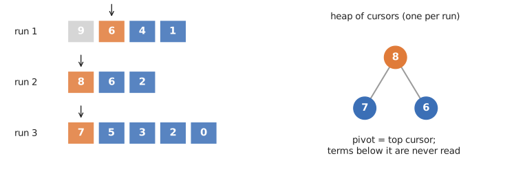
Three runs (columns of D added so far) and a heap of their current heads. Run 1's head (9) cancelled and was skipped; the pivot is now the top cursor, 8.
- Add a column: push one cursor pointing at its head.
- Pop the pivot: take the largest cursor, sum in any other cursors on the same row, and advance them all.
Good
- Nothing below the pivot is ever read. When columns are long and the reduction stops near the top, almost all of each column is skipped.
- The heap has one slot per column added, not per term, so it stays small and in cache.
- It is the only representation that does well on every kind of matrix we have tried, hence the default. On GrPPH it is 3–4× faster than heap columns.
Bad
- Every column of \(D\) must be sorted before it is added. Matrices that can produce their columns already sorted
should say so with
sorted_column, and the cache can keep sorted columns for reuse. - Each step of the pivot search is a heap operation, which costs more than flipping a bit (pivot columns) when columns are dense.
Sorted columns
SortedColumns keeps the working column as one vector, sorted ascending, so the pivot is the last entry.
Columns added are collected unsorted; at the next pivot query they are sorted together (they are usually few and
short) and merged in, starting from their smallest entry: everything below that stays where it is.
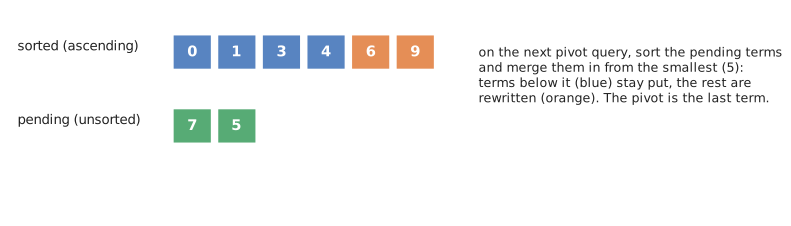
The merge works by position over two slices, which compiles to a tight loop. (An earlier version merged through iterator adaptors and kept its state in memory, which made it twice as slow; the benchmarks caught it.)
Good
- When the columns added stay close to the pivot, so each merge only rewrites the top of the vector: typical of homology of simplicial and cell complexes, where it is the fastest representation (about 1.5× faster than merged columns on Rips homology), and of small dense matrices.
Bad, sometimes very bad
- When the columns added reach far below the pivot: each addition then rewrites nearly the whole working column, so the cost grows with its length. On GrPPH and on the cohomology of cubical complexes it is 15–35× slower than merged columns, and on structured Vietoris–Rips it can take hours where the others take seconds.
Only use it after measuring it on your matrices.
Pivot columns
PivotColumns is PHAT’s bit_tree_pivot_column: the working column is a dense array with a slot for every row,
plus a 64-ary tree of bitsets saying which slots are in use.
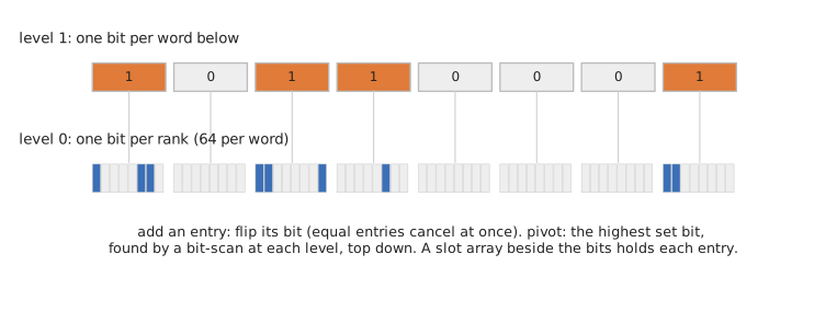
Level 0 has a bit per row (by rank); each bit of level 1 says whether a word of level 0 is non-zero. Three levels cover 262,144 rows, four cover 16 million.
- Add an entry: write it into its slot and flip its bit. Over Z/2 equal entries cancel at once, by the flip. The upper levels only change when a word becomes empty or non-empty.
- Pop the pivot: the highest set bit, found by one bit-scan (a single instruction) per level, from the top down.
This needs the rank of every row in filtration order, so a matrix provides it with row_ranks; for matrices that
don’t, pivot columns fall back to merged columns. (The Python bindings refuse 'pivot' there rather than silently
merging.)
Making it fast
Profiling turned up three things worth knowing, all specific to Z/2:
- Branchless flips. “Is this row already present?” is a coin toss on dense columns, which the CPU mispredicts
constantly. Since a field with one non-zero element is Z/2,
phlitedetects it at compile time (the coefficient type is zero-sized) and flips the bit unconditionally, writing the slot whether or not the entry ends up present. That cut dense 400 × 400 matrices from 28 ms to 11 ms. - Flipping a word at a time. Entries arrive sorted, so neighbours share a 64-bit word; gathering their flips and applying them together avoids each flip waiting on the last one’s write (dense: 8.8 → 7.3 ms).
- No rank lookups. When rows are already numbered by rank (as for explicit complexes),
RowRanks::identityskips the table entirely.
Good
- Many columns added to each, as for explicit dense or cubical complexes, especially with stored R:
1.4–5× faster than merged columns there, and the default for explicit complexes in the Python
phlitepackage.
Bad
- Every entry added is visited: nothing below the pivot is skipped, unlike merged columns.
- A slot for every row, allocated once per reduction: fine for explicit complexes, impossible for Vietoris–Rips (where rows are simplices labelled by huge sparse indices).
- Only serial clearing reuses one working column; the standard and parallel algorithms make a fresh column per column, and use merged columns instead.
Caching columns
Separately from the representation, an algorithm can keep each column of \(D\) the first time it is added,
sorted, in a ColumnCache shared by every column of that dimension (cache_columns). Later additions of the same
column then neither recompute nor re-sort it.
flowchart LR
    A["add column k of D"] --> Q{"in the cache?"}
    Q -- yes --> RUN["sorted run<br/>(shared, Arc)"]
    Q -- no --> GEN["oracle: column(k)"] --> SORT["sort"] --> STORE["cache it"] --> RUN
    RUN --> W["working column"]
The cache is a concurrent map (DashMap), so the parallel algorithm shares it between threads, and it is cleared at
the end of each dimension (columns are only ever added within their dimension).
Good
- When columns are expensive to compute: on GrPPH, whose coboundary enumerates the path cofaces of a digraph,
caching makes merged columns about 3× faster. It is on by default in
phlite_grpphand the Rust library.
Bad
- When columns are cheap: the cache holds every column needed in a dimension until the dimension is done, which
for Vietoris–Rips is most of the memory the reduction uses (23 MB rather than 5 MB for 400 points), and looking a
column up costs about as much as recomputing it. Off in
phlite_rips. - When the matrix stores its columns sorted (
sorted_column, as for explicit complexes): columns are then never sorted, only copied, and the cache saves just that copy. That helps when columns are long (about 10% on cell complexes) and costs a little when they are short (about 20% on cubical complexes). Off in thephlitePython package.
Choosing a representation
Start with the defaults: each package picks the one that won its benchmarks. If you are writing your own oracle:
flowchart TD
    Q1{"can the matrix give<br/>row ranks?"}
    Q1 -- yes --> P["PivotColumns + store_r,<br/>cache off if columns come sorted"]
    Q1 -- no --> Q2{"are columns of D<br/>expensive to compute?"}
    Q2 -- yes --> M["MergedColumns, cached"]
    Q2 -- no --> Q3{"short columns, few<br/>added per column?"}
    Q3 -- yes --> H["HeapColumns, uncached<br/>(least memory)"]
    Q3 -- no --> MU["MergedColumns, uncached"]
| Matrix | Best | Package default |
|---|---|---|
| Vietoris–Rips cohomology | heap or merged, uncached | phlite_rips: heap, uncached |
| GrPPH cohomology | merged, cached | phlite_grpph: merged, cached |
| explicit cubical / dense / cell complexes | pivot, store R, uncached | phlite: pivot, store R, uncached |
| homology of small simplicial complexes | sorted |
All combinations are compared in the benchmarks, and every combination is checked to give the same barcode by the tests.
Bookkeeping: pivot tables and maps
Besides the working column, the clearing algorithm keeps per-column state, all keyed by cell labels:
| Map | Key → value | Used for |
|---|---|---|
pivot table (low_inverse) | pivot row → owner column (and pivot coefficient) | “who owns this pivot?”, on every addition |
| previous pairs | row → column | clearing the next dimension |
| reduction columns | column → \(V_j\) | adding \(R_j = D V_j\), representatives |
| stored R | (a vector, indexed from the pivot table) | storing R |
| essential, skipped births | column | the diagram |
ElementMap: three storages
phlite::bookkeeping::ElementMap chooses its storage from the key type and the value’s size, at compile time:
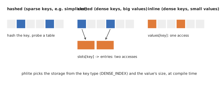
- Hashed (
FxHashMap): for labels without dense indices, such as simplices packed into 64-bit integers. Memory proportional to the entries. - Slotted: for dense labels with large values. A vector of 4-byte slots indexed by the label, pointing into a vector of entries: two memory accesses per lookup, 4 bytes per possible label.
- Inline: for dense labels with values of at most 8 bytes (with their
Optiontag), such as a pivot table over Z/2. The values live in the indexed vector itself: one memory access per lookup.
On large explicit complexes the reduction is limited by memory latency (see where the time goes), so one access instead of two is a real saving.
The owner of a pivot
Finding the column that owns a pivot is the reduction’s most frequent question. The pivot table stores an Owner,
which is either the owning column (whose \(R\) is a column of \(D\), or recomputed from \(V\)) or the position of
its stored column of \(R\), so that adding a stored column is one lookup, not two. Over Z/2 with 4-byte labels the
whole entry (with its Option tag) fits in 8 bytes, so the table is inline; a unit test guards that layout.
Full basis
Normally apparent pairs are not stored in the pivot table, and an owner not found there is recomputed through the transpose (two dependent lookups in the transpose and two in the matrix).
When the table is inline it has a slot for every row anyway, so storing apparent pairs too is free, and then the table
alone answers “who owns this pivot?” in one access. But that is only correct if every column of the dimension is in
the basis: an apparent pair whose column isn’t visited is never recorded. So it is an explicit promise,
Clearing::full_basis(true), which phlite_py makes (its basis is every cell up to some dimension) and the
involution, whose basis is restricted, must not.
flowchart TD
    Q["owner of row r?"] --> T{"in the pivot table?"}
    T -- yes --> O["owner"]
    T -- no --> F{"full basis promised<br/>and table inline?"}
    F -- yes --> N["nobody"]
    F -- no --> A["first column in row r,<br/>is its pivot r?"] --> O2["owner (apparent) or nobody"]
Explicit complexes (phlite_py)
The phlite Python package reduces complexes you give it explicitly, like PHAT and LoPHAT. Under the hood it is an
ordinary phlite oracle over stored matrices, but laid out so that the reduction runs at PHAT’s speed.
Two stages
flowchart LR
    IN["columns, CSC arrays<br/>or Python cells"] --> CH["ChainComplex<br/>validated boundary (CSC),<br/>repeats summed"]
    CH -->|"filtration(values)"| CX["Complex<br/>renumbered by rank,<br/>boundary + coboundary"]
    CX -->|"persistence()"| BC["Barcode<br/>(cells, values, reps)"]
    CH -->|"another filtration"| CX2["another Complex"]
- A
ChainComplexis the boundary matrix in compressed sparse column (CSC) format withu32cell indices, validated (faces one dimension down) and with repeated entries summed. It has no filtration, so one chain complex can be given many. filtration(values)builds aComplex: it checks every face enters no later than its cofaces, then lays the matrices out for the reduction.
Renumbering by rank
The reduction visits cells in filtration order, and looks up rows by their position in that order. If cells kept their
input numbering, every lookup would jump around memory. So a Complex renumbers every cell by its rank, its
position in the order on (value, index):
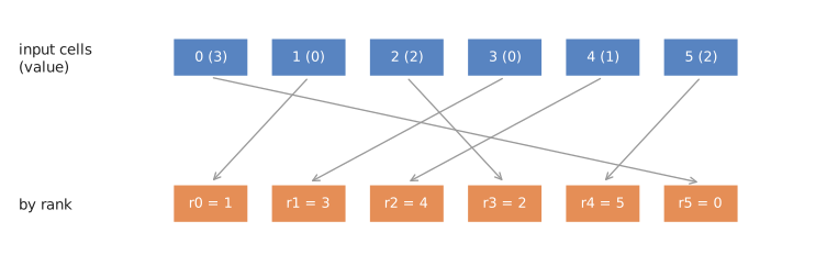
Input cells with values; renumbered by rank (ties broken by index). Results are translated back.
That buys four things:
- The rank is the filtration value. Comparing ranks orders entries exactly as comparing
(value, index)does, so the views use the rank itself (au32) asFiltrationT. The reduction never reads a real value: one random memory access per entry saved, and entries half the size. - Rows are their own ranks, so pivot columns need no rank table (
RowRanks::identity). - Columns are sorted by rank: each column is stored in decreasing rank order, so the pivot is the first entry and
the smallest the last (
column_pivot,column_minandsorted_columnare O(1) or free). - Dense labels:
CellsetsDENSE_INDEX, so all bookkeeping is in vectors, mostly inline.
Since ranks are finer than values, “are these two cells at the same value?” (for skipping zero-length pairs) needs the
real values: a Complex keeps, for each rank, where its run of equal values starts (tie_start), so the check reads
only the later cell, which in a reduction is the column being reduced, in order.
It also stores the transpose (the coboundary), sorted the same way, which gives apparent pairs in O(1) and the involution for representatives.
Results
Bars come out of the reduction in rank space and are turned into records with input cells, values and dimensions in
one pass (a cell’s value, input index and dimension sit together, 16 bytes per rank, so translating a bar reads one
place). Records are small Copy structs, sorted by birth cell with a radix sort. Python objects are only created when
you access the bars.
Memory
Per filtered complex: about 8 bytes per non-zero entry (4 in each of the boundary and coboundary) and 36 bytes
per cell (column pointers for both matrices, the rank tables and the values), with at most 2³² − 2 entries. The
inputs are validated once, in the ChainComplex.
Where the time goes
Two very different regimes show up in practice.
Compute-bound: Rips and GrPPH
For Vietoris–Rips and GrPPH the cost is in producing columns: enumerating cofacets, computing diameters or path lengths, comparing labels. The optimisations that matter are the ones that avoid building columns at all (apparent and emergent pairs, clearing, leaving zero-length pairs out of the basis) and cheap label arithmetic (Rips packs a simplex into one integer and computes its cofacets by inserting a digit; GrPPH compares paths through a packed 128-bit key).
Latency-bound: large explicit complexes
A 1000 × 1000 image (4 million cells) has surprisingly little work: about 2 million columns to look at, 94 thousand that need reducing, and about a million column additions. Its working set (matrices, pivot table, working column) is hundreds of megabytes, far beyond the CPU cache, and each step of the reduction is a chain of dependent random memory accesses: find the pivot, look up its owner, find the owner’s column, read its rows. Each miss costs on the order of 100 ns.
sequenceDiagram
    participant R as reduction
    participant T as pivot table
    participant M as matrix
    R->>T: owner of pivot r?
    T-->>R: column j (miss)
    R->>M: where is column j?
    M-->>R: offset (miss)
    R->>M: rows of column j
    M-->>R: rows (miss)
    Note over R: add them, find the next pivot, repeat
In this regime the number of misses per step is everything, and generality costs misses: a rank lookup, a filtration
value lookup, a two-level map, recomputing an apparent owner through the transpose. Before it was tuned, phlite made
four or five dependent misses per pivot lookup where PHAT makes one, and was 2× slower on such grids. Closing the gap
meant letting explicit complexes declare PHAT-like structure through opt-in hooks:
| Change | Grid 1000 × 1000 (Rust) |
|---|---|
| starting point | 770 ms |
| renumber cells by rank (no change on its own: the misses moved elsewhere) | 779 ms |
| use the rank as the filtration value | 758 ms |
inline maps, apparent pairs in the pivot table (full_basis) | 628 ms |
| identity row ranks (no table lookup) | 505 ms |
| stored R found from the pivot table | 463 ms |
| zero-length checks in order, basis in one pass | 442 ms |
u32 column pointers | 435 ms |
PHAT takes about 400 ms on the same matrix. What remains is mostly phlite doing more: it keeps the transpose too
(for apparent pairs, cohomology and representatives), translates results back to your cells with values, and drops
zero-length bars. On rings images and meshes it is now level with PHAT to within about 10%; on dense matrices and
sparse cell complexes it is level or faster.
Measuring
phlite_py/examples/reduce_file.rs reduces a complex dumped from the benchmark cache, in pure Rust, so you can profile
without Python:
RUSTFLAGS="-C force-frame-pointers=yes" cargo build --release -p phlite_py --example reduce_file
perf record -g target/release/examples/reduce_file grid1000.bin 5
perf stat -e cycles,instructions,LLC-load-misses quickly tells you which regime you are in.
Tutorial: your own filtration in Rust
This tutorial builds persistent homology for a filtration phlite has never seen: the cubical complex of a 3D
greyscale volume (a CT scan, a simulation, a 3D image), with the lower-star filtration: a cell appears with its
brightest voxel. It starts with the least you can implement, and each step adds a piece that unlocks an optimisation.
When is a lazy oracle the right tool?
phlite’s oracles never store the matrix, and that pays off when most of the matrix never needs touching, not
merely when it wouldn’t fit in memory:
- Most pairs are zero-length apparent pairs. In a lower-star filtration nearly every cell is paired with a neighbour that appears at the same moment; in Vietoris–Rips nearly every simplex is. Such cells needn’t be reduced, recorded, or even listed (apparent pairs).
- The top dimension needn’t be enumerated. Cohomology only meets the top cells as rows, produced on demand.
- Columns are cheap to compute from a compact label, so recomputing them costs less than storing them.
Vietoris–Rips complexes often fit in memory, and storing them is still the wrong choice: they are huge, sparse and
almost entirely apparent pairs. The opposite case is a complex where many columns need genuine reduction: dense
boundaries, or cubical complexes of pure noise. There the work is in adding columns, and PHAT’s tricks (dense indices,
pivot columns, storing R) win. For those, build the complex explicitly with the phlite Python package
(which applies all of them), or use PHAT.
A smooth 3D volume is in the lazy camp: in the example below, 94.5% of the cells are in zero-length apparent pairs.
| Step | You implement | You unlock |
|---|---|---|
| 1 | a cell label and a boundary oracle | homology (Betti numbers), standard algorithm |
| 2 | a filtration and a column basis | persistent homology |
| 3 | a coboundary oracle | cohomology and clearing: the top dimension is never listed |
| 4 | (attach the transpose) | apparent pairs |
| 5 | the optional hooks | emergent pairs, cheap apparent pairs |
| 6 | a basis without zero-length apparent pairs | a basis 18× smaller, a quarter of the memory |
| 7 | (attach the transpose; turn on threads) | representatives, parallel reduction |
The code is two examples in the phlite crate, sharing the volume and its geometry:
cargo run --release -p phlite --example volume_basic                       # steps 1–4
cargo run --release -p phlite --example volume_lazy --features parallel    # steps 5–7
The complex
Voxels are vertices. Between two adjacent voxels is an edge, between four a square, between eight a cube. It is convenient to put every cell on a grid twice as fine as the volume: a coordinate that is odd spans two voxels, so a cell’s dimension is its number of odd coordinates. Here is the same idea in 2D:
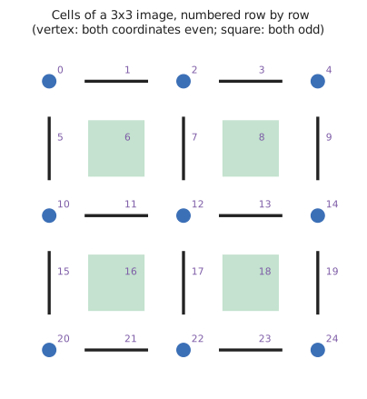
In 2D: a vertex where both coordinates are even, an edge where one is odd, a square where both are. The volume adds a third coordinate.
Numbering the grid point by point gives every cell a u64. A cell’s faces are one step either way along each odd
coordinate, and its cofaces one step either way along each even coordinate, so both are computed from the number
alone. Nothing about the complex is stored but the voxels:
/// Voxels are vertices. The cells sit at the points of a grid of side `2 size - 1`, at coordinates `(x, y, z)`:
/// a coordinate that is odd spans two voxels, so a cell's dimension is its number of odd coordinates (a vertex, an
/// edge, a square or a cube). Cells are numbered `(x · side + y) · side + z`.
impl Volume {
    pub fn side(&self) -> u64 {
        2 * self.size as u64 - 1
    }

    pub fn n_cells(&self) -> u64 {
        self.side().pow(3)
    }

    fn coordinates(&self, cell: u64) -> [u64; 3] {
        let side = self.side();
        [cell / (side * side), (cell / side) % side, cell % side]
    }

    fn number(&self, [x, y, z]: [u64; 3]) -> u64 {
        let side = self.side();
        (x * side + y) * side + z
    }

    pub fn dimension(&self, cell: u64) -> usize {
        self.coordinates(cell).iter().filter(|&&c| c % 2 == 1).count()
    }

    /// The faces of a cell: one step either way along each odd coordinate (at most six).
    pub fn faces(&self, cell: u64) -> impl Iterator<Item = u64> {
        let coords = self.coordinates(cell);
        let mut faces = [None; 6];
        for axis in 0..3 {
            if coords[axis] % 2 == 1 {
                for (k, step) in [-1i64, 1].into_iter().enumerate() {
                    let mut face = coords;
                    face[axis] = (face[axis] as i64 + step) as u64;
                    faces[2 * axis + k] = Some(self.number(face));
                }
            }
        }
        faces.into_iter().flatten()
    }

    /// The cofaces of a cell: one step either way along each even coordinate, inside the grid (at most six), in
    /// increasing order of their numbers: the steps down (along x, then y, then z), then the steps up (z, y, x).
    pub fn cofaces(&self, cell: u64) -> impl Iterator<Item = u64> {
        let coords = self.coordinates(cell);
        let side = self.side();
        let mut cofaces = [None; 6];
        for axis in 0..3 {
            if coords[axis] % 2 == 0 {
                if coords[axis] > 0 {
                    let mut down = coords;
                    down[axis] -= 1;
                    cofaces[axis] = Some(self.number(down));
                }
                if coords[axis] + 1 < side {
                    let mut up = coords;
                    up[axis] += 1;
                    cofaces[5 - axis] = Some(self.number(up));
                }
            }
        }
        cofaces.into_iter().flatten()
    }

    /// The lower-star filtration: a cell appears with its brightest voxel (of the up to eight it spans).
    pub fn value(&self, cell: u64) -> f32 {
        let [x, y, z] = self.coordinates(cell);
        let n = self.size as u64;
        let mut value = f32::NEG_INFINITY;
        for i in [x / 2, x.div_ceil(2)] {
            for j in [y / 2, y.div_ceil(2)] {
                for k in [z / 2, z.div_ceil(2)] {
                    value = value.max(self.voxels[((i * n + j) * n + k) as usize]);
                }
            }
        }
        value
    }
}
The cofaces are produced in increasing order of their numbers, which step 5 puts to use.
1. A boundary matrix
The least phlite needs is a label type for cells and a matrix oracle.
The label
/// A cell of the volume's cubical complex, by its number (see `Volume`).
#[derive(Clone, Copy, Debug, PartialEq, Eq, PartialOrd, Ord, Hash)]
pub struct Cell(pub u64);

// Mark `Cell` as a label for rows and columns. Its order (derived: by number) breaks ties between equal values.
impl BasisElement for Cell {}
BasisElement marks a type as a row or column label. It must be Ord (the order breaks ties between cells with the
same filtration value) and Clone, and it is cloned a lot, so it should be small: here one u64.
The oracle
/// Step 1: the boundary matrix, as an oracle. Nothing is stored: a column is computed when it is asked for.
#[derive(Clone, Copy)]
pub struct Boundary<'a>(pub &'a Volume);

impl MatrixOracle for Boundary<'_> {
    type CoefficientField = Z2;
    type ColT = Cell;
    type RowT = Cell;

    fn column(&self, col: Cell) -> impl Iterator<Item = (Z2, Cell)> {
        self.0.faces(col.0).map(|face| (Z2::one(), Cell(face)))
    }
}
Three associated types say what the matrix is over (Z2, whose one non-zero element is zero-sized) and what labels
its columns and rows; column returns an iterator over a column’s entries. The boundary is computed from the cell’s
number each time: the oracle holds just a reference to the volume.
Running it
To reduce a matrix, phlite also needs the order on rows and which columns to reduce, in that order. With
no filtration, with_trivial_filtration() puts every cell at time 0, so rows are ordered by label alone, and the
basis must list the columns in the same order:
/// The columns to reduce: every cell up to dimension `max_dim`, by dimension, each in the order of the rows. With no
/// filtration that is just the order on labels: by number.
fn basis_by_number(volume: &Volume, max_dim: usize) -> SplitBasis<Cell> {
    let mut dims: Vec<Vec<Cell>> = vec![vec![]; max_dim + 1];
    for cell in 0..volume.n_cells() {
        let dim = volume.dimension(cell);
        if dim <= max_dim {
            dims[dim].push(Cell(cell));
        }
    }
    SplitBasis::from_dimensions(dims)
}
// Step 1: no filtration (every cell at time 0): every finite bar has length zero, so only the essential ones are
// left, which count the holes of a solid cube: one component, and nothing else
let d = Boundary(&volume).with_trivial_filtration();
let d = d.with_basis(basis_by_number(&volume, 3));
let betti = barcode::homology(&d, Algorithm::Standard(Standard::new()), false);
println!("No filtration: {}", summary(&volume, &betti));barcode::homology reduces the boundary with the standard algorithm. With every cell at
time 0, every finite bar has length zero and is dropped, which leaves the essential bars: the Betti numbers of a solid
cube.
No filtration: 1 bars in H0, 0 in H1 and 0 in H2
The basis must be in the rows’ order. The first version of this example sorted the basis by voxel value while the rows, with no filtration, were ordered by number. The reduction then pairs the wrong cells, and this example reported thousands of loops and cavities in a solid cube.
phlitecan’t check the order for you without visiting every column, so this is worth a test of its own.
You can now compute the homology of anything you can describe cell by cell.
2. A filtration and a basis
For persistent homology the rows need filtration values. Implement HasRowFiltration on the oracle:
/// Step 2: the filtration on rows (cells), read off the volume. Implementing it on the oracle, rather than attaching
/// a closure with `with_filtration`, leaves room to override the optional hooks later.
impl HasRowFiltration for Boundary<'_> {
    type FiltrationT = NotNan<f32>;

    fn filtration_value(&self, row: Cell) -> NotNan<f32> {
        NotNan::new(self.0.value(row.0)).unwrap()
    }
}
The filtration type must be Ord; NotNan from ordered-float is the usual choice. (For a quick experiment you can
attach a closure instead, with Boundary(&volume).with_filtration(|cell| ...), but implementing the trait on your own
type leaves room for the optional hooks in step 5.)
Rows are now ordered by (value, label), so the basis must be too:
/// As `basis_by_number`, but in filtration order: by value, then number.
fn basis(volume: &Volume, max_dim: usize) -> SplitBasis<Cell> {
    let mut dims: Vec<Vec<Cell>> = vec![vec![]; max_dim + 1];
    for cell in 0..volume.n_cells() {
        let dim = volume.dimension(cell);
        if dim <= max_dim {
            dims[dim].push(Cell(cell));
        }
    }
    for cells in &mut dims {
        cells.sort_by_key(|&cell| (NotNan::new(volume.value(cell.0)).unwrap(), cell));
    }
    SplitBasis::from_dimensions(dims)
}
// Step 2: the lower-star filtration, by homology, with the standard algorithm.
// Every cell, cubes included, is a column.
let d = Boundary(&volume).with_basis(basis(&volume, 3));
let standard = timed("homology, standard algorithm", || {
barcode::homology(&d, Algorithm::Standard(Standard::new()), false)
});
println!(" {}", summary(&volume, &standard));The result is a list of Bars: birth cell and value, death cell and value (None if essential), and optionally a
representative.
You can now compute persistent homology. But the standard algorithm reduces every column, cubes included, and builds every column in full. On a 40³ volume (493,039 cells) that takes 5.4 s.
3. Cohomology and clearing
The coboundary lists each cell’s cofaces. Its oracle mirrors the boundary’s:
/// Step 3: the coboundary matrix (the transpose of the boundary), with the same filtration.
#[derive(Clone, Copy)]
pub struct Coboundary<'a>(pub &'a Volume);

impl MatrixOracle for Coboundary<'_> {
    type CoefficientField = Z2;
    type ColT = Cell;
    type RowT = Cell;

    fn column(&self, col: Cell) -> impl Iterator<Item = (Z2, Cell)> {
        self.0.cofaces(col.0).map(|coface| (Z2::one(), Cell(coface)))
    }
}

impl HasRowFiltration for Coboundary<'_> {
    type FiltrationT = NotNan<f32>;

    fn filtration_value(&self, row: Cell) -> NotNan<f32> {
        NotNan::new(self.0.value(row.0)).unwrap()
    }
}
and now cohomology with clearing is available:
    // Step 3: cohomology with clearing. Columns stop at the squares (for H0, H1 and H2): the cubes only ever appear
    // as rows, cofaces of squares, and are never enumerated
    let delta = Coboundary(&volume).with_basis(basis(&volume, 2));
    let cohomology = timed("cohomology, clearing", || {
        barcode::cohomology(&delta, Algorithm::Clearing(Clearing::new()))
    });
Two things changed:
- The basis stops at the squares. For \(H_0\), \(H_1\) and \(H_2\) by cohomology the columns are vertices, edges and squares; cubes only appear as rows, produced by the oracle as cofaces of squares. They are never listed.
- Clearing.
barcode::cohomologyreverses the coboundary (the anti-transpose) and reduces it dimension by dimension, skipping every column that the previous dimension’s pairs show to be zero. The basis must be split by dimension, whichSplitBasisis.
On the 40³ volume this takes 157 ms, against 5.4 s for the standard algorithm on the boundary: 34× faster.
You can now use every algorithm in phlite that doesn’t need extra information about the matrix.
4. Apparent pairs
The boundary is the coboundary’s transpose, and attaching it costs one line:
    // Step 4: attach the transpose, so that apparent pairs need no reduction, and zero-length ones aren't recorded
    let delta_t = (&delta).with_transpose(Boundary(&volume));
    let apparent = timed("cohomology, clearing, apparent pairs", || {
        barcode::cohomology(&delta_t, Algorithm::Clearing(Clearing::new()))
    });
With the transpose the reduction can ask “which is the first column with an entry in row \(r\)?” (the smallest entry of column \(r\) of the transpose), and so recognise apparent pairs: pairs that need no reduction and no storage. In a lower-star filtration most pairs are apparent, and most of those have length zero (an edge and its brighter end appear together), which clearing then doesn’t even record.
But measure it:
A 40³ volume: 493039 cells

homology, standard algorithm                    5375.1 ms
cohomology, clearing                             156.7 ms
cohomology, clearing, apparent pairs             186.4 ms
Here it is 20% slower. Our columns have at most six entries, so reducing a column is cheap anyway, and the transpose’s generic answer (scan the column of the transpose, computing every entry’s filtration value from up to eight voxels) costs more than it saves. Apparent pairs pay off when a column is expensive to reduce, or, as in the next two steps, when they can be recognised more cheaply and used to avoid listing cells at all.
This is a general lesson: every optimisation in phlite has a cost, and the only way to know whether it pays on
your matrix is to time it.
5. The optional hooks: emergent pairs
HasRowFiltration has optional methods (hooks) with correct but generic defaults. Overriding them tells the
reduction things about your matrix that it would otherwise work out the slow way. volume_lazy.rs starts from the
filtration order on cells, and the two questions apparent pairs ask:
/// The filtration order on cells: by value, then number.
fn key(volume: &Volume, cell: u64) -> (NotNan<f32>, u64) {
    (NotNan::new(volume.value(cell)).unwrap(), cell)
}

/// The oldest coface of a cell (the first column in its row of the boundary), and its youngest face (its pivot).
fn oldest_coface(volume: &Volume, cell: u64) -> Option<u64> {
    volume.cofaces(cell).min_by_key(|&c| key(volume, c))
}

fn youngest_face(volume: &Volume, cell: u64) -> Option<u64> {
    volume.faces(cell).max_by_key(|&f| key(volume, f))
}
and overrides three hooks on the coboundary:
impl HasRowFiltration for Coboundary<'_> {
    type FiltrationT = NotNan<f32>;

    fn filtration_value(&self, row: Cell) -> NotNan<f32> {
        NotNan::new(self.0.value(row.0)).unwrap()
    }

    // Step 5, emergent pairs: cohomology's pivot of a column is its *smallest* coface. No coface comes before the cell
    // itself, and cofaces are enumerated in increasing order of their numbers, so the first coface with the cell's own
    // value is the smallest: stop there. Most columns need nothing else, so this usually looks at one or two cofaces.
    fn column_min(&self, col: Cell) -> Option<ColumnEntry<NotNan<f32>, Cell, Z2>> {
        let own = self.filtration_value(col);
        let mut best: Option<ColumnEntry<NotNan<f32>, Cell, Z2>> = None;
        for coface in self.0.cofaces(col.0) {
            let entry: ColumnEntry<_, _, _> = (Z2::one(), Cell(coface), self.filtration_value(Cell(coface))).into();
            if entry.filtration_value == own {
                return Some(entry);
            }
            if best.as_ref().is_none_or(|b| entry < *b) {
                best = Some(entry);
            }
        }
        best
    }

    // Step 5, apparent pairs without the transpose: the columns with an entry in row `r` of the coboundary are the
    // faces of `r`, so the first and last are its oldest and youngest faces
    fn first_column_in_row(&self, row: Cell) -> Option<Cell> {
        self.0.faces(row.0).min_by_key(|&f| key(self.0, f)).map(Cell)
    }

    fn last_column_in_row(&self, row: Cell) -> Option<Cell> {
        youngest_face(self.0, row.0).map(Cell)
    }
}column_min: emergent pairs. Cohomology reduces the reversed coboundary, whose pivot is a column’s smallest coface. In a lower-star filtration no coface can come before the cell itself, and our cofaces come in increasing order of their numbers, so the first coface with the cell’s own value is the smallest, and the search stops there. Most columns need nothing but their pivot (nobody else owns it), so most columns are finished after looking at one or two cofaces. Ripser does the same for Vietoris–Rips; Bauer calls these emergent pairs.first_column_in_row/last_column_in_row: apparent pairs without the transpose. The columns with an entry in row \(r\) of the coboundary are exactly the faces of \(r\), so the first is its oldest face. No transpose, and no adding up of coefficients.column_pivotisn’t overridden: homology would use it, cohomology doesn’t.
Every hook must be right. A pivot that isn’t the true smallest entry, or a “first column” that isn’t, gives a wrong barcode silently. The example checks its barcode against the other methods; the property tests show how to test hooks against their defaults on random inputs.
    // Step 5: the hooks find pivots (emergent pairs) and apparent pairs without building columns or the transpose.
    // Columns are cheap to compute, so recompute them rather than caching, and keep the working column as a heap
    let algorithm = Clearing::new().with_columns(HeapColumns).cache_columns(false);
    reset_peak_memory();
    let full = timed("build every cell up to dimension 2", || full_basis(&volume, 2));
    let delta_full = Coboundary(&volume).with_basis(full);
    let hooks = timed("cohomology, clearing, hooks", || {
        barcode::cohomology(&delta_full, Algorithm::Clearing(algorithm.clone()))
    });
On their own the hooks don’t buy much here: on the 40³ volume this runs in 167 ms, about the same as plain clearing in step 3. With at most six cofaces per column, stopping the search early saves little. (For Vietoris–Rips, where a simplex can have thousands of cofacets, emergent pairs are what make cohomology fast.) What the hooks do buy is cheap, exact apparent pairs, which the next step builds on.
Heap columns, uncached, as in phlite_rips: our columns are short and cheap to recompute, so there is nothing to
gain from sorting or keeping them (see choosing a representation).
6. Leaving cells out
This is where a lazy oracle pulls ahead of a stored matrix. A cell in a zero-length apparent pair needs no
reduction and gives no bar, and the reduction can recognise it again as an owner when it needs it (through
first_column_in_row). So it needn’t be in the basis at all:
/// Step 6: whether a cell is in a zero-length apparent pair, as either its birth or its death. Such cells needn't be
/// in the basis at all: the reduction finds them again as owners (through `first_column_in_row`) when it needs them.
fn in_zero_apparent_pair(volume: &Volume, cell: u64) -> bool {
    let value = volume.value(cell);
    // A birth: its oldest coface has the same value, and the cell is that coface's youngest face
    let birth = oldest_coface(volume, cell)
        .is_some_and(|coface| volume.value(coface) == value && youngest_face(volume, coface) == Some(cell));
    // A death: its youngest face has the same value, and the cell is that face's oldest coface
    let death = youngest_face(volume, cell)
        .is_some_and(|face| volume.value(face) == value && oldest_coface(volume, face) == Some(cell));
    birth || death
}

/// The columns to reduce, up to dimension `max_dim`, without the cells of zero-length apparent pairs. Cells are
/// streamed (never all held at once), so memory goes on the cells that are kept.
fn reduction_basis(volume: &Volume, max_dim: usize) -> SplitBasis<Cell> {
    let mut dims: Vec<Vec<Cell>> = vec![vec![]; max_dim + 1];
    for cell in 0..volume.n_cells() {
        let dim = volume.dimension(cell);
        if dim <= max_dim && !in_zero_apparent_pair(volume, cell) {
            dims[dim].push(Cell(cell));
        }
    }
    for cells in &mut dims {
        cells.sort_by_key(|&cell| key(volume, cell.0));
    }
    SplitBasis::from_dimensions(dims)
}
A cell is in a zero-length apparent pair as a birth if its oldest coface has the same value and has it as youngest face, or as a death if its youngest face has the same value and has it as oldest coface. Both checks are local: a few voxel lookups. Cells are streamed, so only those kept are ever stored.
    // Step 6: leave the cells of zero-length apparent pairs out of the basis altogether
    let reduced = timed("build the reduction basis", || reduction_basis(&volume, 2));
    let reduced_size = basis_size(&reduced);
    let delta = Coboundary(&volume).with_basis(reduced);
    let lazy = timed("cohomology, clearing, reduction basis", || {
        barcode::cohomology(&delta, Algorithm::Clearing(algorithm.clone()))
    });
    println!(
        "    basis: {reduced_size} cells instead of {full_size} ({:.1}%)",
        100.0 * reduced_size as f64 / full_size as f64
    );
    if let (Some(full), Some(lazy)) = (full_peak, peak_memory_mb()) {
        println!("    peak memory: {lazy:.0} MB instead of {full:.0} MB");
    }
On a 96³ volume (7 million cells, 6.1 million of them up to dimension 2):
build every cell up to dimension 2                    2965.6 ms
cohomology, clearing, hooks                           3017.3 ms
build the reduction basis                             2211.4 ms
cohomology, clearing, reduction basis                 2020.2 ms
    basis: 338183 cells instead of 6110496 (5.5%)
    peak memory: 78 MB instead of 326 MB
The basis is 18× smaller, the reduction 1.5× faster, and peak memory a quarter. Building the basis is now the
largest cost, and it is embarrassingly parallel (phlite_rips builds its basis on all cores).
For comparison, storing this complex explicitly, as PHAT or the phlite Python package do, takes about 36 bytes per
cell and 8 per boundary entry, roughly 400 MB here, before any reduction.
Trade-offs
- Only the clearing algorithms can leave cells out: the standard algorithm needs every column.
- The test must be exactly right: leave out a cell that isn’t in a zero-length apparent pair and its bar is lost.
- It pays when most pairs are zero-length apparent pairs (lower-star filtrations of smooth data, Vietoris–Rips). On noise, where few pairs have length zero, the test costs more than it saves.
7. Representatives and threads
Two last things come almost for free.
    // Step 7: representatives, by the involution, which needs the transpose (the boundary)
    let delta_t = (&delta).with_transpose(Boundary(&volume));
    let with_reps = timed("... with representatives", || {
        barcode::cohomology_with_involution(&delta_t, Algorithm::Clearing(algorithm.clone()))
    });
    let longest = with_reps
        .iter()
        .filter(|bar| volume.dimension(bar.birth.0) == 2 && bar.death.is_some())
        .max_by_key(|bar| bar.death.unwrap().1 - bar.birth_value)
        .expect("a finite cavity");
    println!(
        "    the longest finite H2 bar, [{}, {}), is a closed surface of {} squares",
        longest.birth_value,
        longest.death.unwrap().1,
        longest.representative.as_ref().unwrap().len()
    );

    // ... and all cores
    #[cfg(feature = "parallel")]
    let parallel = timed("cohomology, parallel clearing", || {
        let parallel = Clearing::new()
            .with_columns(HeapColumns)
            .cache_columns(false)
            .parallel();
        barcode::cohomology(&delta, Algorithm::ParallelClearing(parallel))
    });
Representatives
barcode::cohomology_with_involution computes the pairs by cohomology and then cycle representatives by a small
homology reduction of just the death and essential birth columns (the involution). It
needs the boundary, attached as the transpose. Each Bar’s representative is a list of (coefficient, cell): for a
bar in \(H_2\), a closed surface of squares enclosing a dark cavity in the volume.
... with representatives                              4121.2 ms
    the longest finite H2 bar, [0.536, 0.632), is a closed surface of 1268 squares
Threads
Clearing::new().parallel() (feature parallel) reduces each dimension on all cores
(parallel clearing):
cohomology, parallel clearing 1575.0 ms
(against 2020 ms on one thread, on a laptop with four cores). The reduction itself is a small part of the work here, since most columns finish at their pivot.
What not to turn on
phlite also has PHAT’s tricks: dense indices for vector bookkeeping,
pivot columns and stored R. They need an array over every cell,
which is exactly what this oracle avoids, and they pay when many columns need genuine reduction, which isn’t the
case here. If your complex is like that, build it explicitly with the phlite Python package,
which applies them all.
Next
The same ideas, applied to Vietoris–Rips with much more care over enumerating cofacets, are phlite_rips; its source
(phlite_rips/src/lib.rs onwards, comments marked TUTORIAL) is a good next read.
The three Python packages
| Package | Crate | Input | Typical use |
|---|---|---|---|
phlite | phlite_py | a chain complex you build: integer columns, CSC arrays, or your own cell objects; any filtration | cubical complexes, simplicial complexes, cell complexes, anything PHAT or LoPHAT would take |
phlite_rips | phlite_rips | a distance matrix | Vietoris–Rips persistence, like ripser and giotto-ph |
phlite_grpph | phlite_grpph | a weighted digraph (networkx or edge list) | grounded persistent path homology, like grpphati |
The full API reference (every class, method and argument) is generated from the packages’
docstrings with Sphinx (docs/python). These chapters are the guide.
All three share:
- an
Algorithmclass, with the same options, to choose the reduction; method="cohomology"(default) or"homology";representatives=Truefor a cycle representing each bar;- release of the GIL during the computation, so other Python threads keep running.
Installing
The packages are built from source with maturin. From a crate’s directory:
just develop # builds the release extension into the current virtual environment
or with maturin directly: maturin develop --release -m phlite_py/Cargo.toml.
Barcodes at a glance
import phlite

chain = phlite.ChainComplex.from_pairs([(0, []), (0, []), (1, [0, 1])])
barcode = chain.filtration([0.0, 1.0, 2.0]).persistence()
barcode.pairings      # [(1, 2)]: the component born at cell 1 dies at cell 2
barcode.essential     # [0]
barcode.diagram(0)    # array([[0., inf], [1., 2.]])
from phlite_rips import rips
barcode = rips(distances, max_dim=1, representatives=True)
barcode.pairings[1]                  # (birth, death) values of the finite H1 bars
barcode.pairing_representatives[1]   # a cycle (list of edges) for each
phlite‘s barcode is in terms of cells (with diagram for values); phlite_rips’ and phlite_grpph’s are lists
per dimension of values, with representatives as lists of simplices or paths.
phlite: explicit complexes
The phlite package computes persistence of a filtered chain complex you build yourself. There are three steps:
flowchart LR
    A["ChainComplex<br/>from_pairs / from_columns /<br/>from_csc / from_cells"] -->|".filtration(values)"| B["FilteredComplex"]
    B -->|".persistence(...)"| C["Barcode"]
    A -->|".filtration(other values)"| B2["another FilteredComplex"]
1. Build a chain complex
A ChainComplex is the cells, their dimensions and their boundaries, with no filtration. It is validated once.
import phlite

# A hollow triangle on vertices 0, 1, 2, filled in by cell 6
pairs = [
    (0, []), (0, []), (0, []),        # vertices
    (1, [0, 1]), (1, [1, 2]), (1, [0, 2]),  # edges
    (2, [3, 4, 5]),                   # the triangle
]
chain = phlite.ChainComplex.from_pairs(pairs)
| Constructor | Takes | Notes |
|---|---|---|
from_pairs(pairs) | [(dimension, boundary), ...] | as PHAT and LoPHAT |
from_columns(boundaries, dimensions) | two lists | |
from_csc(indptr, indices, dimensions, data=None) | numpy arrays | the fast path: no per-entry Python objects |
from_cells(cells, ...) | your own objects (or tuples) with a dimension and a boundary | results come back as your objects |
All take coefficients= (per boundary entry) and modulus= (2, 3, 5, 7, 11 or 13).
Your own cells. Any hashable object with a dimension and a boundary() works (the same protocol as grpphati’s
Column), or plain values with functions saying how to get the pieces:
chain = phlite.ChainComplex.from_cells(
    simplices,                                   # tuples of vertices
    dimension=lambda s: len(s) - 1,
    boundary=lambda s: {s[:i] + s[i + 1:]: (-1) ** i for i in range(len(s))} if len(s) > 1 else {},
    modulus=3,
)
For large complexes of your own objects, key= (an injective map to integers) matches cells in Rust instead of
through Python hashing, from_key= avoids storing the objects at all, and face_keys=True lets boundary return
face keys rather than face objects (usually the real speed-up, since building face objects is the slow part).
2. Attach a filtration
filtered = chain.filtration([0, 0, 0, 1, 1, 2, 3]) # one value per cell
Cells enter in order of value, ties broken by index; every face must enter no later than its cofaces (otherwise a
ValueError names the offending cells). values can be a sequence or numpy array (fastest), a mapping from cells
to values, a function of a cell, or omitted (cells’ entrance_time, else their order). With extend=True missing
values are filled in as the maximum over the faces, so values on vertices give the lower-star filtration.
One chain complex can be filtered many times, cheaply: the validation and indexing are done once.
3. Compute persistence
barcode = filtered.persistence(
    max_dim=None,            # default: the top dimension
    method="cohomology",     # or "homology"
    algorithm=None,          # an Algorithm, default Algorithm.serial()
    representatives=False,
)
The Barcode is in terms of your cells:
bars | every bar: dimension, birth, death, birth_value, death_value, persistence, is_essential, representative |
pairings, essential | (birth, death) cells of finite bars, births of infinite ones |
bar(cell), representative(cell) | the bar born at a cell |
diagram(dim), diagrams() | (k, 2) numpy arrays of (birth, death) values, inf for essential bars |
Representatives are (cell, coefficient) lists in decreasing filtration order, so the birth cell comes first. Bars of
length zero are omitted (with the default index filtration there are none, so you get every pair, as with PHAT).
Performance
The explicit complexes chapter explains how a filtered complex is laid out. Against PHAT’s twist reduction, on one thread with the matrix prebuilt:
| input | random | structured (long bars) |
|---|---|---|
| Rips complexes, by cohomology | phlite 7–10× faster | phlite 9–13× faster |
| cubical complexes | PHAT 1.1–1.2× faster | PHAT 1.2–1.3× faster |
| triangulated surfaces | level to PHAT 1.1× faster | |
| sparse cell complexes | phlite 1.1–2× faster | |
| dense boundaries | level |
See the notebooks for worked examples: an image, a point cloud’s alpha-like complex, and a lower-star filtration on a mesh.
phlite_rips: Vietoris–Rips
import numpy as np
from phlite_rips import rips, Algorithm

points = np.random.default_rng(0).normal(size=(100, 2))
distances = np.linalg.norm(points[:, None] - points[None], axis=-1)

barcode = rips(distances, max_dim=1, representatives=True)
barcode.pairings[1]                  # [(birth, death), ...] of the finite H1 bars
barcode.essential[0]                 # births of the infinite H0 bars
barcode.pairing_representatives[1]   # a cycle (a list of edges (a, b)) for each finite H1 bar
| Argument | Default | |
|---|---|---|
distance_matrix | a square numpy array (float64 or float32) or nested list; inf means the edge never appears | |
max_dim | the highest homology dimension | 1 |
threshold | only build simplices up to this diameter (bars alive then become essential) | None |
method | "cohomology" or "homology" | "cohomology" |
algorithm | an Algorithm | Algorithm.serial() (heap columns, uncached) |
representatives | compute a cycle for every bar | False |
What it does
It implements the optimisations of Ripser and giotto-ph on phlite’s oracles:
- Simplices as integers. A simplex’s vertices are the digits of a base-\((n+1)\) number, so a simplex is one
usize, and its cofacets and facets are computed arithmetically by inserting or removing a digit. - Clearing and cohomology by default.
- Emergent pairs: cofacets are enumerated in order, and the first with the simplex’s own diameter is its pivot, so most columns are finished after a step or two.
- Zero-length apparent pairs are left out of the basis entirely (they are nearly all of them), and the basis is built in parallel for the parallel algorithm.
- Truncation at the enclosing radius (beyond it the complex is a cone), and an optional threshold.
- Heap columns, uncached by default: Rips columns are cheap to recompute, and caching them dominates the memory.
On point clouds with long bars (noisy spheres, wedges of circles), merged cached columns
(
Algorithm.serial().with_columns("merged").with_cache(True)) are up to 1.9× faster at about twice the memory. Avoid'sorted'columns on such inputs: they can take hours.
See the notebooks for a circle, a torus and representatives drawn on the points.
phlite_grpph: path homology of digraphs
Grounded persistent path homology (Chaplin, Harrington and Tillmann) is a persistence theory for weighted digraphs
that sees directed cycles: a directed square, a long directed loop, a bidirected edge. phlite_grpph computes it, with
representatives, much faster than the reference implementation grpphati.
import networkx as nx
from phlite_grpph import grpph

G = nx.DiGraph()
G.add_weighted_edges_from([("a", "b", 1.0), ("b", "c", 1.0), ("c", "d", 1.0), ("d", "a", 1.0)])

barcode = grpph(G, representatives=True)
barcode.pairings[1]                  # [(0.0, 2.0)]: the directed 4-cycle, filled in at distance 2
barcode.pairing_representatives[1]   # [[('d', 'a'), ('c', 'd'), ('b', 'c'), ('a', 'b')]]
barcode.essential[0]                 # [0.0]: one component
or with integer nodes: grpph(4, [(0, 1, 1.0), (1, 2, 1.0), (2, 3, 1.0), (3, 0, 1.0)]).
| Argument | Default | |
|---|---|---|
graph, edges | a networkx DiGraph / MultiDiGraph, or a node count and (source, target, weight) edges | |
weight | the edge attribute holding weights (missing means 1) | "weight" |
method | "cohomology" or "homology" (homology needs every 2-cell up front: far more memory) | "cohomology" |
algorithm | an Algorithm | Algorithm.serial() (merged columns, cached) |
representatives | a cycle for every bar, as a list of nodes (H0) or edges (H1) | False |
What it does
The filtration is the grounded path complex: edges of the graph are present from time 0 (so the cycle above is born at 0, not at 1), and the regular path complex of the shortest-path digraph grows with distance. Its coboundary enumerates the allowed paths extending a path, which is relatively expensive, so:
- columns of the coboundary are cached (sorted) once per dimension: about 3× faster;
- merged columns keep the working column small and never read below the pivot: 3–4× faster than heap columns;
- paths are compared through a packed 128-bit key instead of a nested enum.
The cost grows with the number of nodes (the shortest-path digraph is complete), so keep graphs to a few hundred nodes; edges are cheap.
See the notebooks for a worked example with directed cycles.
Choosing an algorithm
Each package has an Algorithm class (phlite.Algorithm, phlite_rips.Algorithm, phlite_grpph.Algorithm), built
from the same code, whose presets use the package’s own defaults.
from phlite import Algorithm

Algorithm.serial()                          # the default
Algorithm.parallel(threads=8)
Algorithm.clearing().with_columns("heap").with_cache(True)
Start from a preset or an algorithm, then adjust with with_* methods (each returns a new Algorithm):
| Start from | Is |
|---|---|
Algorithm.serial() | Algorithm.clearing(): clearing, skipping zero-length apparent pairs |
Algorithm.parallel(threads=None) | Algorithm.parallel_clearing().with_threads(threads): parallel clearing on all cores by default |
Algorithm.standard() | the standard algorithm |
| Option | What | phlite | phlite_rips | phlite_grpph |
|---|---|---|---|---|
with_columns | the column representation: 'merged', 'heap', 'sorted', 'pivot' | 'pivot' ('merged' for standard and parallel) | 'heap' | 'merged' |
with_cache | cache columns of the boundary | False | False | True |
with_store_r | store R (serial clearing only) | True | False | False |
with_skip_zero_apparent_pairs | skip zero-length apparent pairs | True (not for standard) | ||
with_dimension_order | reduce dimensions in this order (clearing) | detected | ||
with_storage | 'locking' or 'lock-free' (parallel) | 'locking' | ||
with_threads | thread count (parallel) | all cores |
Options an algorithm can’t use are errors, not ignored: with_threads on serial(), or 'pivot' columns on the
parallel algorithm or in phlite_rips and phlite_grpph (whose matrices have no row ranks).
Every option is visible. The repr lists every resolved option, as a chain that rebuilds it:
>>> phlite.Algorithm.serial()
Algorithm.clearing().with_columns("pivot").with_cache(False).with_store_r(True).with_skip_zero_apparent_pairs(True)
>>> phlite_rips.Algorithm.parallel(4)
Algorithm.parallel_clearing().with_columns("heap").with_cache(False).with_skip_zero_apparent_pairs(True).with_storage("locking").with_threads(4)
and each option is a property (.columns, .cache, .store_r, …).
Every algorithm gives the same barcode; only the time and memory differ. The defaults won their package’s benchmarks; see choosing a representation for when to change them.
Example notebooks
These are marimo notebooks, in docs/notebooks/, each published with its outputs as a page of its own (the links below). Each draws
the dataset, its barcode and representatives (with Altair), and ends with an animation of the filtration: the complex
growing on the left, and on the right the barcode with the bars alive at that moment highlighted. To run one yourself, and change it, open it in the environment with the
package installed:
cd python-tests
uv run --project latest --group docs marimo edit ../docs/notebooks/phlite_image.py   # phlite notebooks
uv run --group docs marimo edit ../docs/notebooks/rips_points.py                     # phlite_rips and phlite_grpph
An image (phlite)
The cubical complex of a 64 × 64 image with three dark rings, built from Python tuples, with the lower-star filtration
from pixel values (extend=True). The representatives of the three longest H1 bars trace the rings.
A Delaunay complex (phlite)
Two noisy circles, their Delaunay triangulation filtered by edge length, over Z/3: a few hundred simplices instead of the Rips complex’s millions, and the same two loops.
Vietoris–Rips (phlite_rips)
A noisy figure eight: its two loops, drawn from their representatives, and a few algorithm configurations timed.
A digraph (phlite_grpph)
Directed cycles of different lengths, two parallel paths and a bidirected edge: grounded persistent path homology tells them apart, and each representative is highlighted on the graph.
Testing
Every algorithm, representation and option must give the same barcode, and that is what most of the tests check, from three directions: against reference libraries, against invariants that need no reference, and component by component.
Against references (Python, Hypothesis)
python-tests/ generates random inputs with Hypothesis, which shrinks a failure
to a minimal example.
- Explicit complexes (
test_sparse.py): random cellular complexes over Z/2 (multi-edges, loops, empty and long boundaries, few distinct values so many ties) against PHAT and LoPHAT, for every configuration in the grid (algorithm × columns × caching × skipping × dimension order × store R × threads × storage), both methods, every input format. - Vietoris–Rips (
test_rips.py): random distance matrices (point clouds, small-integer matrices with ties, infinite entries) against ripser and giotto-ph. - GrPPH (
test_grpph.py): random weighted digraphs against grpphati.
Invariants (no reference needed)
test_invariants.py uses cellular complexes over Z/2, Z/3 and Z/5 with cells listed out of filtration order, and
checks properties every barcode must have, with exact linear algebra over Z/p (tests/modp.py):
- The rank invariant: for values \(s \le t\), the bars alive from \(s\) to \(t\) number \(\dim(Z_d(K_s) + B_d(K_t)) - \dim B_d(K_t)\). This alone determines the barcode. (Also for Rips.)
- Betti numbers and the Euler characteristic from the essential bars.
- Representatives are cycles in the right dimension, led by the birth cell, that become boundaries exactly at the death.
- Invariance: relabelling cells, strictly increasing changes of values (and of distances for Rips, weights for GrPPH) change the bars accordingly.
- Bar structure, and agreement between the barcode’s accessors.
Components (Rust, proptest)
- Every column representation, driven through the whole column API by random operations, against a plain map from
row to coefficient (Z/2 and Z/3, with and without row ranks, through
reverse()). ElementMapandElementSetagainstBTreeMapandBTreeSet, for every storage.- phlite_py’s renumbering by rank and every clearing configuration on random simplicial complexes.
Running them
just test            # everything, briefly (100 examples per Hypothesis test)
just fuzz 20000      # 20000 cases per property test and examples per Hypothesis test (~40 minutes)
Every test has a time limit (pytest-timeout), so a bug that makes a reduction loop forever fails the run rather than
hanging it.
Were they worth it?
The fuzz tests have found real bugs: a panic for dimension orders beyond the matrix, births of skipped pairs reported as essential under some dimension orders, and wrong representatives when a restricted basis met the single-lookup pivot table (see full basis). Deliberately reintroduced bugs in the bit tree, the “same value” check and coefficient cancellation are all caught.
Benchmarks
The full, regenerated results are in
python-tests/BENCHMARKS.md, with time
and peak memory for every configuration. The suites:
| Suite | phlite package | Against | Inputs |
|---|---|---|---|
bench_rips.py | phlite_rips | ripser, giotto-ph | random points in a cube; noisy torus, sphere, wedges of circles and spheres |
bench_grpph.py | phlite_grpph | grpphati | random digraphs; rings and lattices |
bench_sparse.py | phlite | PHAT, LoPHAT | Rips complexes, cubical complexes of noise and of an image of rings, a meshed torus, sparse and dense cell complexes |
Each benchmark checks its barcode against the reference before timing, records peak memory (with memray, so Rust allocations are counted), and runs its first round in a forked process with a time limit, so one pathological configuration can’t stall a whole session.
Headline results, one thread:
- Vietoris–Rips: on a par with ripser and giotto-ph; faster in dimension 2 on random points. The default (heap columns, uncached) favours memory; merged cached columns are up to 1.9× faster on point clouds with long bars, at about twice the memory.
- GrPPH: 25–100× faster than grpphati.
- Explicit complexes, against PHAT’s twist reduction with a prebuilt matrix: 7–13× faster on Rips complexes, 1.1–2× faster on sparse cell complexes, level on dense boundaries and meshes, PHAT 1.1–1.3× faster on cubical complexes.
just bench           # every benchmark
just bench-check     # compare the quick cases with the saved baselines
just bench-docs      # rerun everything and regenerate BENCHMARKS.md
References
- U. Bauer. Ripser: efficient computation of Vietoris–Rips persistence barcodes. J. Appl. Comput. Topol. 5 (2021). Clearing with cohomology, apparent and emergent pairs, recomputing columns.
- U. Bauer, M. Kerber, J. Reininghaus, H. Wagner. PHAT – Persistent Homology Algorithms Toolbox. J. Symb. Comput. 78 (2017). Twist reduction, bit-tree pivot columns.
- C. Chen, M. Kerber. Persistent homology computation with a twist. EuroCG (2011). Clearing.
- T. Chaplin, H. A. Harrington, U. Tillmann. Grounded persistent path homology: a stable, topological descriptor for weighted digraphs. Found. Comput. Math. (2024).
- M. Čufar. Ripserer.jl: flexible and efficient persistent homology computation in Julia. JOSS 5 (2020). Involuted persistence for representatives.
- V. de Silva, D. Morozov, M. Vejdemo-Johansson. Dualities in persistent (co)homology. Inverse Problems 27 (2011).
- H. Edelsbrunner, J. Harer. Computational Topology: An Introduction. AMS (2010).
- H. Edelsbrunner, D. Letscher, A. Zomorodian. Topological persistence and simplification. Discrete Comput. Geom. 28 (2002). The standard algorithm.
- D. Morozov, A. Nigmetov. Towards lockfree persistent homology. SPAA (2020). The parallel reduction.
- N. Otter, M. A. Porter, U. Tillmann, P. Grindrod, H. A. Harrington. A roadmap for the computation of persistent homology. EPJ Data Science 6 (2017).
- J. Pérez, S. Hauke, U. Lupo, M. Caorsi, A. Dassatti. giotto-ph: a Python library for high-performance computation of persistent homology of Vietoris–Rips filtrations. arXiv:2107.05412 (2021). Parallel apparent pairs and bases.