Persistent homology in one chapter
This chapter recaps just enough persistent homology to follow the algorithms, through one running example. For a proper introduction see Edelsbrunner and Harer’s Computational Topology, or Otter et al.’s A roadmap for the computation of persistent homology (see references).
Filtrations
A filtered chain complex is a chain complex whose cells appear one at a time. Each cell has a filtration value (the time it appears), and every face of a cell must appear no later than the cell itself. Here is the running example: four vertices, five edges and a triangle.

The running example. At t = 4 the triangle abc fills in the loop a–b–c.
Listing the cells by filtration value (breaking ties by a fixed order), we get a filtration order:
| index | 0 | 1 | 2 | 3 | 4 | 5 | 6 | 7 | 8 | 9 |
|---|---|---|---|---|---|---|---|---|---|---|
| cell | a | b | c | ab | bc | ac | d | cd | bd | abc |
| value | 0 | 0 | 1 | 1 | 1 | 2 | 2 | 3 | 3 | 4 |
Persistence
As cells appear, homology classes (connected components in dimension 0, loops in dimension 1, voids in dimension 2, …) are born and later die. Each class gives a bar from its birth to its death: the barcode.
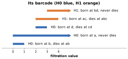
The barcode: two components and a loop die; one component and one loop never do.
Reading it off the filtration:
aandbare born at 0; the edgeabmerges them at 1, so one of the two components dies (by convention the younger one,b).cis born at 1 and dies at 1, whenbcjoins it to the rest: a bar of length zero, which is not drawn.accloses the loop a–b–c at 2; the triangleabcfills it at 4.dis born at 2 and dies at 3.bdcloses another loop at 3 (b–c–d), which nothing ever fills: an essential (infinite) bar.
Persistence by matrix reduction
The boundary matrix \(D\) has a column and a row for every cell, in filtration order; column \(j\) holds the faces of cell \(j\). Over \(\mathbb{Z}/2\) the entries are just 0 and 1.
The pivot (or low) of a column is its last non-zero entry: the face that appeared most recently. We reduce \(D\) by adding columns left to right until no two columns share a pivot, recording the additions in \(V\), so that
\[ R = D V \]
with \(V\) upper triangular. Then the pairing can be read straight off \(R\):
- if column \(j\) of \(R\) has pivot \(i\), the class born at cell \(i\) dies at cell \(j\): a pair \((i, j)\);
- if column \(j\) of \(R\) is zero, cell \(j\) gives birth to a class; if no column has pivot \(j\), that class never dies (it is essential).
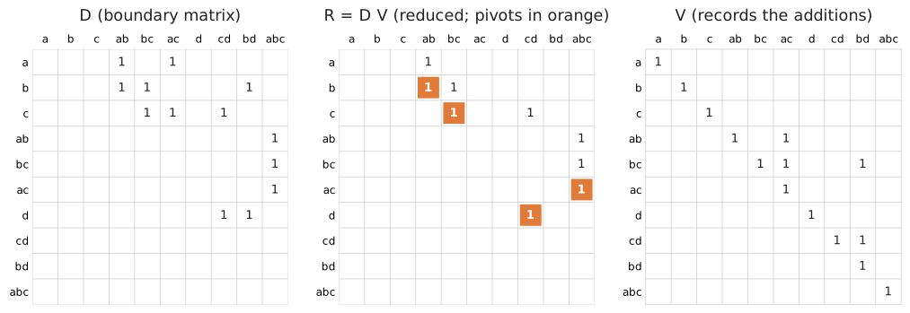
D, its reduction R = DV (pivots in orange) and V. The pairs are (b, ab), (c, bc), (d, cd) and (ac, abc).
Different reductions give different \(R\) and \(V\), but always the same pairs (the pairing uniqueness lemma).
That is what lets phlite choose freely between algorithms, column representations and orders of work: they all
give the same barcode.
Columns of \(R\) and \(V\) are also representatives: for a pair \((i, j)\), column \(j\) of \(R\) is a cycle born at \(i\) that becomes a boundary at \(j\); for an essential class born at \(i\), column \(i\) of \(V\) is a cycle born at \(i\).
Reducing a column
Reducing one column means repeatedly finding its pivot and, if an earlier column owns the same pivot, adding that
column. Here is column ac:
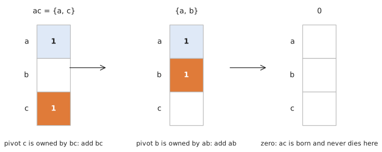
Reducing ac: two additions, after which it is zero, so ac gives birth to a loop.
Every algorithm in phlite is built from these two operations: pop the pivot and add a column. How they are done
is the subject of the column representations; which columns get reduced, and in what
order, is the subject of the reduction algorithms.
Representing a filtration in phlite
phlite doesn’t need you to number your cells or store \(D\). Cells can be labelled by any type (a simplex packed
into an integer, a path in a digraph, a pair of pixel coordinates), and the filtration order is the order on
(filtration value, label). Columns are produced on demand by your oracle.